Learning with Constraints
Reinforcement Learning as a field has advanced in lockstep with advances in compute power. Iterative generation of tricks improved performance by learning the values of actions. The value function is therefore necessary for choosing actions.
Policy Gradient methods are premised on the idea that a policy that selects actions can be learned without a value function.
For vanilla policy gradients (such REINFORCE), the objective used to optimize the neural network looks like:
$$L^{PG}(\theta) = \hat{\mathop{\mathbb{E}}}_t[log \pi{\theta}(a_t|s_t) \hat{\mathop{\mathbb{A}}}_t]$$
where the $\hat{\mathop{\mathbb{A}}}$ could be the discounted return (as in REINFORCE) or the advantage function (as in GAE) for example. Taking a gradient ascent step on this loss with respect to the network parameters incentivizes our agent to pursue actions that led to higher reward.
The vanilla policy gradient method uses the log probability of your
action $(log \pi(a|s))$ to trace the impact of the actions (i.e. credit
assignment), but you could imagine using another function to do this,
for instance a function that uses the probability of the action under
the current policy $(\pi(a|s))$, divided by the probability of the
action under your previous policy $(\pi_{old}(a|s))$, looking like:
$$rt(\theta) = \frac{\pi{\theta}(at|s_t)}{\pi{\theta_{old}}(a_t|s_t)}$$
This expression is greater than 1 when when $a_t$ is more probable for the current policy than it is for the old policy; it will be between 0 and 1 when the $a_t$ is less probable for the current policy than for the old. So, given a difference in rewards between a current policy and an old one, the actions that are more probable under the current policy than the old one receive higher credit for the difference.
If the action is much more probable under the current policy, $r_t(\theta)$ might be so large it leads to taking extremely large/catastrophic gradient steps. To stabilize these effects, Proximal Policy Optimization (PPO) proposes 2 mechanisms: PPO-CLIP and PPO-Penalty.
PPO-CLIP
The Clipped Surrogate Objective function is specified as:
$$L^{CLIP}(\theta) = \hat{\mathop{\mathbb{E}}}_t[ min(r_t(\theta) \hat{\mathop{\mathbb{A}}}_t, clip(r_t(\theta), 1-\epsilon, 1+\epsilon)\hat{\mathop{\mathbb{A}}}_t]$$
The clipping parameter, $\epsilon$ is chosen to bound the $r_t$ value. For instance, if $\epsilon$ is 0.2, then $r_t$ can vary between 0.8 and 1.2.
This variant is the more popular variance of the two, as it does not explicitly have a constraint, but rather uses its clipping hyperparameter to minimize the maximum distance between the proposed new policy and the current policy.
PPO-Penalty
The other variant of PPO penalizes large changes in the policy via a penalty parameter for the KL divergence between the two policies. This penalty coefficient adapts over the course of training to achieve some target value of divergence. The target divergence used is another hyperparameter to be tuned.
$$L^{KLPenalty}(\theta) = \hat{\mathop{\mathbb{E}}}t[ \frac{\pi{\theta}(a_t|s_t)}{\pi_{\theta_{old}}(a_t|s_t)} \hat{\mathop{\mathbb{A}}}_t - \beta KL[\pi_{\theta_{old}}(.|s_t), \pi(.|s_t) ]]$$
Costs
In some environments, agents will pursue actions that we not only want to disincentivize, but actively want to punish. In RL, such simulated settings broadly aim to model real-world scenarios with high-risk and consequences. Agents, in their pursuit of ever-higher returns, must take into account both the rewards they accrue from pursuing the goal and the costs they incur from the path to the goal they pursue. Treating rewards and costs separately allows the world-designer more degrees of freedom for shaping behavior.
The objective functions we have seen above for policy gradient methods allow for parametrizing a cost function in the objective function. However, I instead chose to set a parameter called a cost limit, which can be interpreted as a cost allowance we grant to the agent in the pursuit of its goal. The cost limit is agnostic, in that there could be different costs associated with different safety infractions, and the algorithm does not orient the agent towards one or the other, just tries to minimize the sum total of costs incurred. The algorithm works as follows:
- Collect a set of trajectories by running policy $\pi_k = \pi(\theta_k)$ in the environment.
- Compute the rewards $\hat{R}_k$
- Compute advantage estimates $\hat{A}_t$ (I use Generalized Advantage Estimation but you can use any method), based on the current value function $V{\psi_k}$
- Update the policy by maximizing the PPO Clip objective (or PPO-Penalty, or both)
- Calculate penalized reward: $$R^{PEN} = R - \zeta Cost $$ given penalty coefficient $\zeta$
- Update Penalty Coefficient $\zeta$, $$\zeta{k+1} = max(0, \zeta_k + \lambda{\zeta}(Avg Cost - Cost_{lim} )$$
- Fit the value function by regression with MSE loss, via stochastic gradient descent.
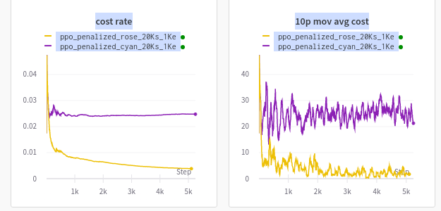
Here is an example of two agents trained in OpenAI Safety Gym’s Point-Goal v1 environment. From the setup specified above, agents learn to limit their costs near the chosen hyperparameter. Are you able to guess which are the two cost limits I used in the experiments below? You may hover over the image for the answer.
